Paper Analysis on LESS: Label-Efficient Semantic Segmentation for LiDAR Point Clouds
In this blog article, I will review of the paper titled LESS: Label-Efficient Semantic Segmentation for LiDAR Point Clouds authored by Minghua Liu, Yin Zhou, Charles R. Qi, Boqing Gong, Hao Su, and Dragomir Anguelov. The paper was published in ECCV 2022.
I will begin by giving a brief overview of the paper. After that, I will discuss related works. Then, I will explain the proposed method and present the desired experiments and comparison results. Finally, I will conclude by summarizing the findings and discussing potential future works, using the proposed method.
Table of Contents
- 1. Introduction
- 2. Related works
- 3. Method
- 4. Experiments
- 5. Conclusion and feature works
- 6. References
- 7. Annex
1. Introduction
1.1 Why LiDARs?
Light detection and ranging (LiDAR) sensors have become a crucial component in autonomous vehicles. They offer more accurate depth measurements and are more reliable under different lighting conditions when compared to visual cameras.
Semantic segmentation plays a vital role in processing LiDAR point clouds. It enables a detailed understanding of the environment, which complements object detection. For example, semantic segmentation helps autonomous vehicles distinguish between drivable and non-drivable road surfaces. It also provides valuable information about parking areas and sidewalks, which are currently not fully detectable by modern object detectors.
1.2 Benchmark datasets and latest approaches
Based on public benchmark datasets for autonomous driving [1][2], I have noticed the emergence of various LiDAR semantic segmentation techniques. These approaches have been developed and refined from these large-scale datasets [3][4][5].
Among the notable methods, there are several latest approaches such as cylindrical and asymmetrical LiDAR segmentation, which aim to improve the accuracy and precision of the segmentation process. Additionally, there is the range-point-voxel fusion LiDAR segmentation method, which combines different data representations to enhance the overall segmentation performance. Another noteworthy technique is the attentive feature fusion with adaptive feature selection for semantic segmentation, which focuses on effectively combining and selecting features to achieve more accurate results. These advancements demonstrate the ongoing efforts to enhance the capabilities of LiDAR-based semantic segmentation in autonomous driving scenarios.
1.3 Point cloud annotations are costly
Typically, these methods require fully labeled point clouds during training. However, labeling all points exhaustively is an extremely laborious and time-consuming task, especially considering that a LiDAR sensor can perceive millions of points per second.
Furthermore, this approach may face scalability issues when expanding the operational domain to include different cities and weather conditions. It may also struggle to cover rare cases effectively.
Most of these methods typically rely on fully labeled point clouds for training purposes. However, manually labeling all points extremely laborious and time-consuming task. This becomes particularly challenging considering that a LiDAR sensor can capture millions of points per second.
Moreover, labeling approach may encounter scalability problems when trying to extend the operational domain to encompass various cities and weather conditions. Additionally, it may struggle to effectively handle rare cases or scenarios that occur less frequently. These challenges highlight the need for more efficient and scalable labeling methods to overcome these limitations in LiDAR-based semantic segmentation.
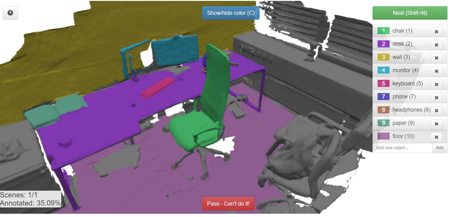
Sample point cloud labeling process
1.4 Label-efficient approaches are important
To scale up the system, label-efficient approaches for LiDAR semantic segmentation play a crucial role. The main objective is to minimize the reliance on human annotations while still achieving high performance in the segmentation task.
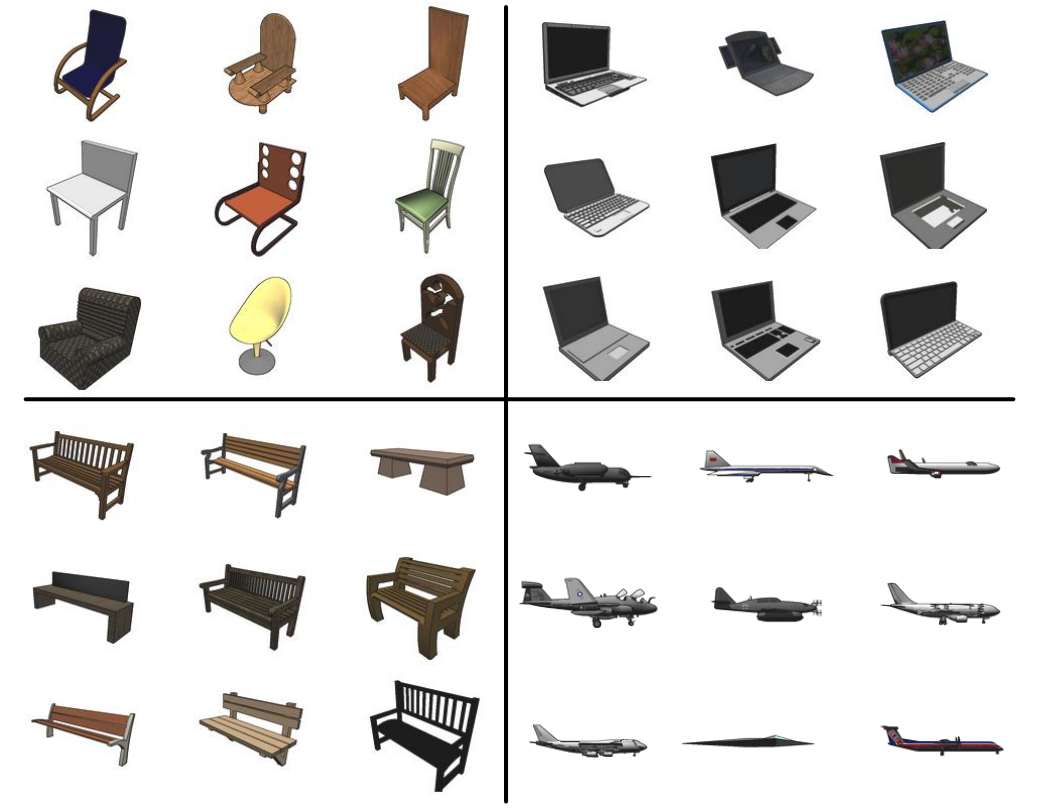
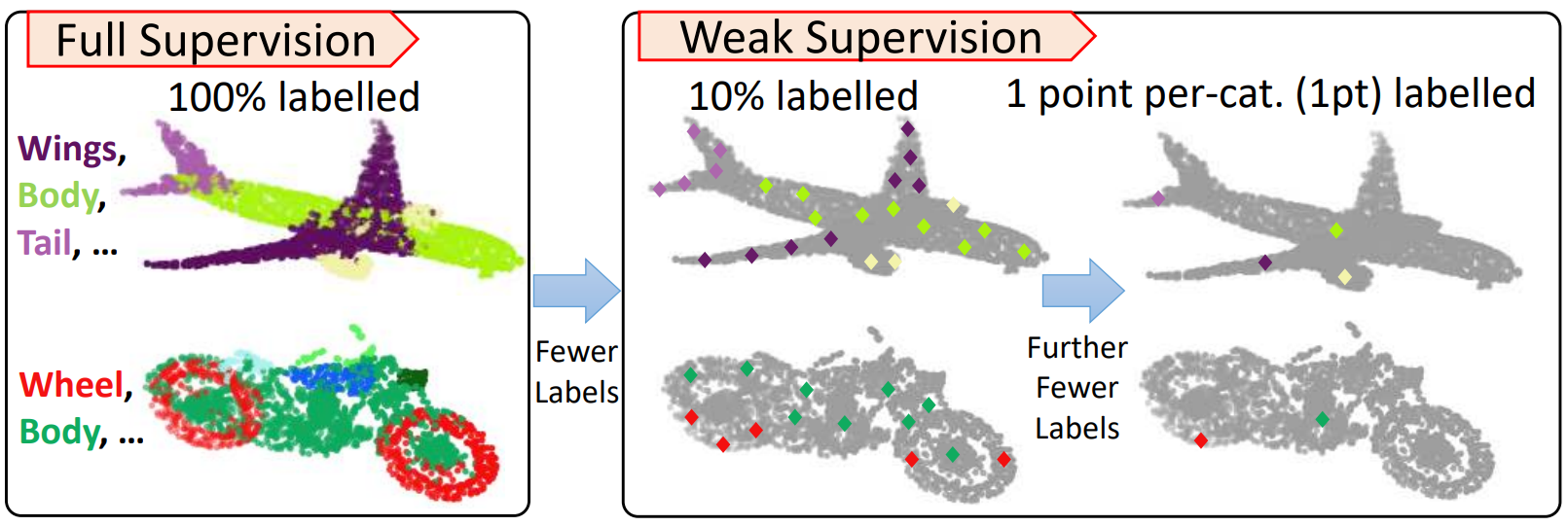
When examining previous studies on label-efficient semantic segmentation, it is worth noting that most of them have primarily focused on indoor scenes [6] or 3D object parts [7]. However, it is crucial to consider that these scenes exhibit notable differences in terms of point cloud appearance and object type distribution when compared to outdoor driving scenes. Outdoor environments introduce significant variations in point density, imbalanced point counts between common types such as ground and vehicles, as well as less common types like cyclists and pedestrians. These unique characteristics pose additional challenges that need to be addressed when developing label-efficient approaches for outdoor LiDAR semantic segmentation.
2. Related works
2.1 Segmentation networks for LiDAR point clouds
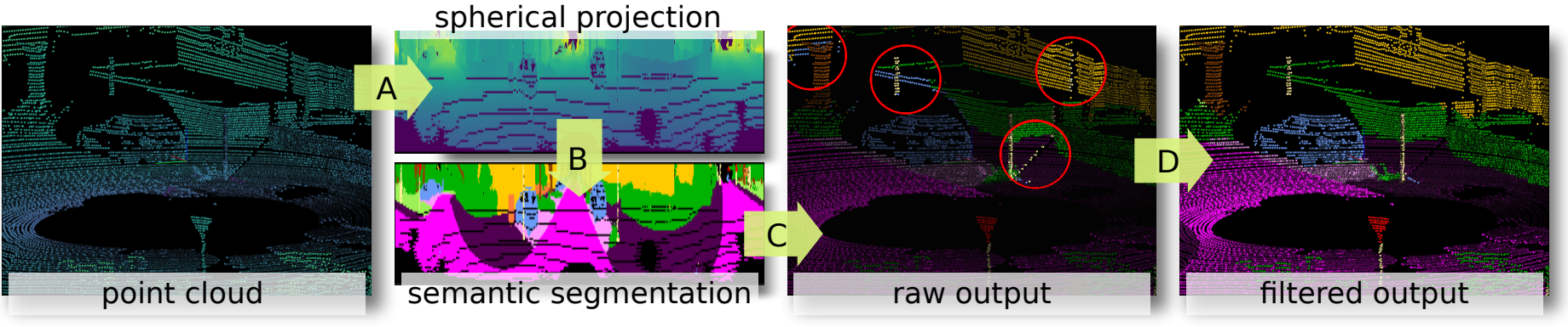
We can say that, outdoor LiDAR point clouds exhibit distinct characteristics, including larger scales, varying densities, and sparsity. These factors pose challenges that require more efficient segmentation networks to be developed. To address this, many approaches have emerged that tackle the issue by projecting 3D point clouds onto 2D images from a spherical view [8] (i.e., range images) or a bird’s-eye view.
Additionally, some method directly process the point clouds without transforming them into other representations, such as images or voxel grids [9]. These approaches aim to streamline the segmentation process by working directly with the point cloud data.
In our paper, we specifically focus on the Cylinder3D backbone as our main research emphasis. This backbone utilizes a voxel-based representation and reduces the computational burden by leveraging cylindrical partition and sparse asymmetrical convolution.
All of these approaches mentioned have the potential to serve as the backbone network in our label-efficient framework, contributing to the development of more efficient and accurate LiDAR semantic segmentation systems.
2.2 Label-efficient 3D semantic segmentation (labeling part)
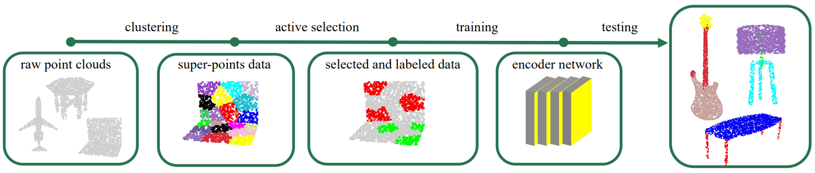
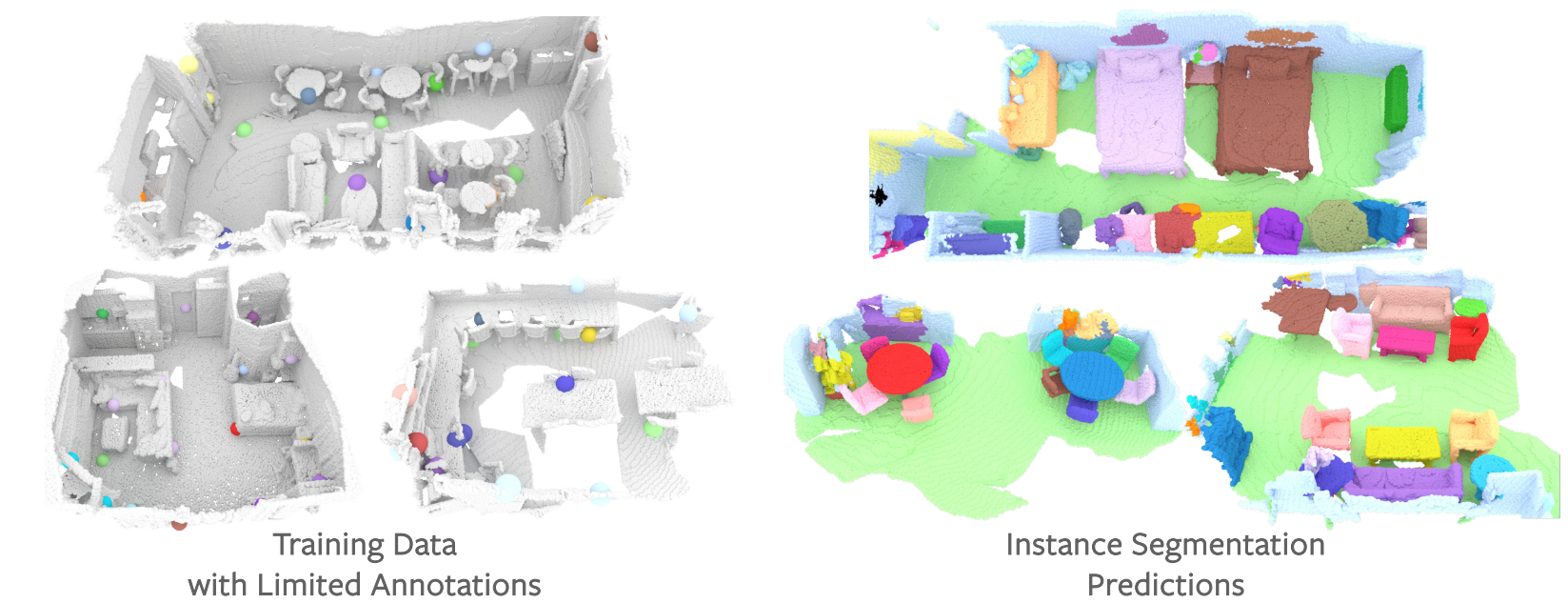
It is certain that there is growing interest in label-efficient 3D semantic segmentation. Specifically, when it comes to labeling, there are various approaches that incorporate active learning [10]. This iterative process involves selecting and requesting specific points to be labeled during the network training phase.
One notable approach, as introduced by Hou et al. [11], involves utilizing features obtained from unsupervised pre-training. These features guide the selection of points that require labeling. In the left image, only the colored points (enlarged for better visibility) are labeled as training samples. The right image displays the predictions made on the validation set, with different colors representing different instances.
There are other methods that involve projecting the point clouds onto a 2D plane and leveraging 2D supervision signals. Some approaches also make use of weak labels at the scene-level or sub-cloud-level. Furthermore, several methods incorporate rule-based heuristics or employ handcrafted features to assist with the annotation process. These strategies contribute to the development of more efficient labeling techniques for 3D semantic segmentation tasks.
2.3 Label-efficient 3D semantic segmentation (training part)
As recent investigations, there are various notable approaches for the training phase. One such approach, as introduced by Xie et al. [11], involves the utilization of contrastive learning for unsupervised pre-training. This technique proves to be effective in improving the training process.
Additionally, some methods employ self-training techniques to generate pseudo-labels. This strategy helps in utilizing unlabeled data to augment the training set [12].
In the context of label propagation, many works incorporate Conditional Random Fields (CRFs) [13] or random walk algorithms to propagate labels. These techniques contribute to refining the segmentation results by leveraging contextual information.
Furthermore, there are several approaches that utilize a combination of different techniques to enhance the training process. These include prototype learning, siamese learning, temporal constraints, smoothness constraints, attention mechanisms, cross-task consistency, and synthetic data. Each of these strategies aims to improve the model’s performance and generalization abilities.
However, it is worth noting that most of the recent studies have primarily focused on indoor scenes or 3D object parts. As a result, there is a significant gap in research when it comes to exploring and addressing challenges in outdoor scenarios. This highlights the need for further exploration and development of techniques specific to outdoor environments.
3. Method
3.1 LESS’s co-design
As a differ from the previous works, this approach involves the co-design of the labeling process and model learning, guided by two key principles:
-
The labeling step is designed to provide minimal supervision, ensuring compatibility with state-of-the-art semi/weakly supervised segmentation methods. The goal is to reduce the annotation effort required while still achieving accurate segmentation results.
-
The model training step utilizes the labeling policy as a prior knowledge, incorporating it into the learning process to derive additional learning targets. This allows for enhanced training and improved performance.
One significant advantage of the proposed method is its seamless integration with most state-of-the-art LiDAR segmentation backbones. It does not require any changes to the network architecture or introduce extra computational complexity when deployed onboard. This makes it highly practical and efficient for effective labeling and learning from scratch.
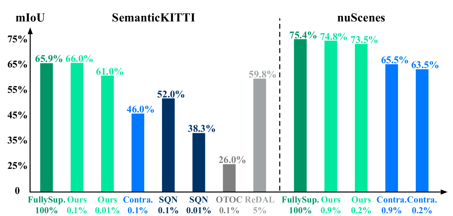
Compared mIoU results of the proposed method and existed methods
Mean Intersection over Union (mIoU) is widely using using evaluation metric in semantic segmentation tasks. This metric is commonly used to assess the accuracy of a segmentation model by measuring the overlap between predicted and ground truth regions.
To calculate mIoU, we first compute the Intersection over Union (IoU) for each class separately. This is done by determining the ratio of the intersection of the predicted and ground truth regions to their union. By taking the average IoU across all classes, we obtain the mIoU value, which provides an overall measure of segmentation accuracy.
The IoU metric serves as an indicator of how well the predicted segmentation aligns with the ground truth. A higher IoU score indicates a better level of segmentation accuracy, indicating a strong alignment between the predicted and ground truth regions. This metric helps in quantitatively assessing the performance of segmentation models in semantic segmentation tasks.
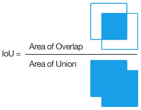
Source: Kaggle
If we analyzing the figure provided, it becomes clear that the proposed method showcases performance levels that closely resemble those of the fully-supervised counterpart. This achievement is remarkable considering that only a mere 0.1% of the SemanticKITTI dataset was used for annotation. Moreover, the proposed method demonstrates comparable performance to other existing methods on the nuScenes dataset.
To provide further context, the ratio between the utilized labels and all points is indicated below each bar in the figure. It is worth emphasizing that all other label-efficient methods being compared primarily concentrate on indoor settings and are not specifically tailored for outdoor LiDAR segmentation. This distinction highlights the significance and novelty of the proposed method in addressing outdoor segmentation challenges effectively.
3.2 Indoor vs Outdoor settings
Generally, previous studies have predominantly concentrated on label-efficient 3D semantic segmentation using indoor datasets like ScanNet-v2 and S3DIS. These datasets are characterized by densely and uniformly distributed points sampled from high-quality meshes. Additionally, objects found in indoor scenarios often exhibit similar sizes and a balanced distribution among different classes.
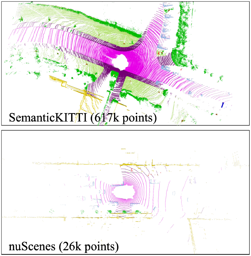
However, when shifting our focus to outdoor settings, we encounter a higher level of complexity. Outdoor driving scenes present challenges such as varying point density and frequent occlusions. Unlike indoor scenarios, the distribution of samples across different categories in outdoor scenes is highly unbalanced. This can be observed from the point distribution figure provided below, where there are significant variations in the number of points belonging to each category. This discrepancy underscores the unique difficulties involved in outdoor 3D semantic segmentation tasks compared to their indoor counterparts.
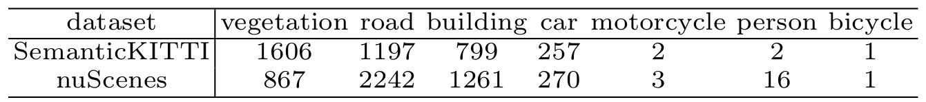
Point distribution across the most common and rarest categories of SemanticKITTI and nuScenes. Numbers are normalized by the sample quantity of bicycles.
The extremely unbalanced distribution adds extra difficulty for label-efficient segmentation, whose goal is to only label a tiny portion of points.
3.3 Pilot study
In my pilot study, authors conducted training experiments with the Cylinder3D semantic segmentation network using the SemanticKITTI dataset by proposing three different setups to evaluate the performance:
-
The first setup involved training the network using 100% labeled points from the dataset, ensuring that every point was annotated.
-
In the second setup, we randomly select and annotate only 0.1% of the points per scan. This means that for each scan, a small percentage of points were labeled for training.
-
The third setup focused on randomly selecting 0.1% of the scans from the dataset and annotating all the points within those selected scans. This approach ensured that a small fraction of the scans were fully annotated for training purposes.
By examining the results of these experiments, we aimed to gain insights into the impact of different annotation strategies on the performance of the Cylinder3D network in the task of semantic segmentation.
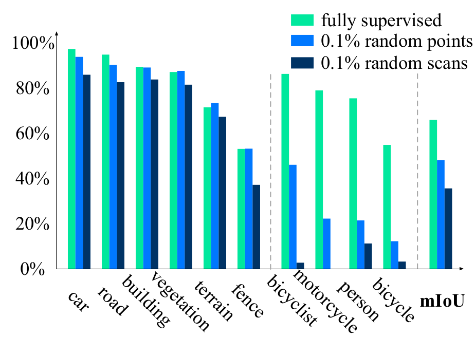
mIoU performance of the most common and rarest categories on SemanticKITTI
Surprisingly, the experimental results show that even with minimal annotation efforts, the setup involving “0.1% random points” achieved a mean Intersection over Union (IoU) of 48.0%. In comparison, the fully supervised version obtained a higher mean IoU of 65.9%.
While the performance on commonly occurring categories remained close to that of the fully supervised model, there were noticeable performance gaps for underrepresented categories such as bicycles, persons, and motorcycles. These categories, characterized by their small sizes and infrequent occurrences, were more affected by the constraints of the reduced annotation budget. However, it is important to note that these categories hold significant importance in the context of autonomous driving.
Interestingly, the authors observed that the “0.1% random points” setup outperformed the “0.1% random scans” setup by a significant margin. This outcome can primarily be attributed to the greater diversity of labeled points obtained in the former approach.
Based on their findings, the authors suggest reevaluating the current approach to label-efficient segmentation. Rather than solely focusing on improving labeling efficiency or training techniques, they propose a co-design approach. By integrating both aspects, we can effectively cover underrepresented instances with limited labeling resources and leverage the efforts put into labeling during network training. This approach has the potential to enhance the performance of label-efficient segmentation systems in handling challenging scenarios.
3.3 LESS’s pipeline
The proposed LESS framework, which integrates pre-segmentation, labeling, and network training processes. One of the significant advantages of this framework is its compatibility with existing LiDAR segmentation backbones. It allows for the integration of the LESS framework without requiring any modifications to the network architectures or causing additional inference latency. This makes the LESS framework highly practical and efficient for incorporating into various LiDAR segmentation systems.
The figure explanation illustrates the following steps:
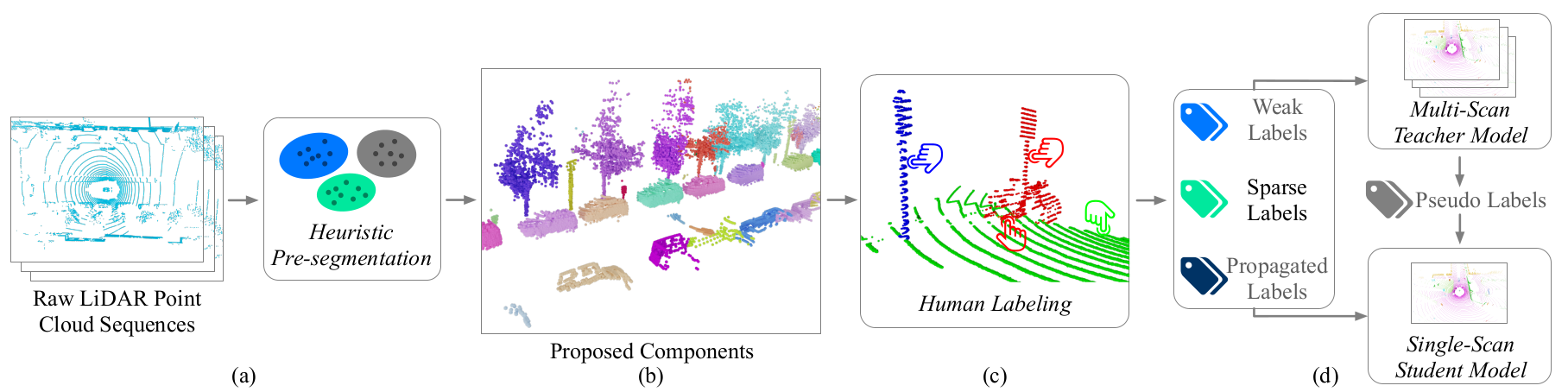
LESS pipeline
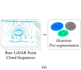
-
We first initially employ a heuristic algorithm to pre-segment each LiDAR sequence into distinct connected components. This step helps in separating and identifying different regions within the LiDAR data.
-
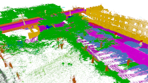
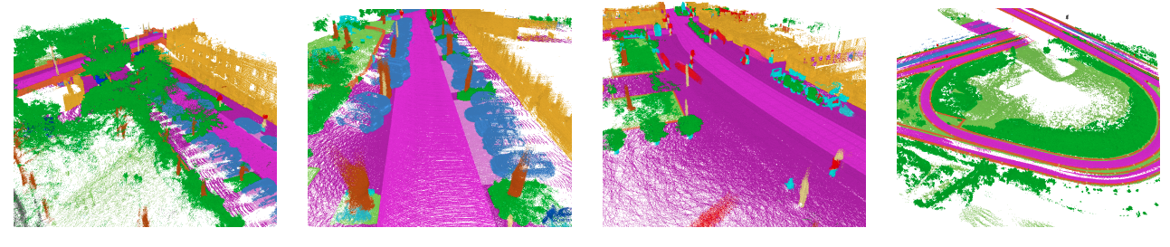
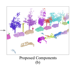
To provide a clear visualization, I present examples of the proposed components, with different colors representing different components. It’s worth noting that components of ground points are not showing to maintain clear visualization.
-
During the labeling process, human annotators are only required to provide coarse labels for each component. Each color in the visual representation corresponds to a proposed component, and the labeled points are indicated by click icons. The focus is on annotating sparse labels directly by humans, reducing the annotation effort while still capturing crucial information.
-
Subsequently, the network is trained to process and interpret the various labels. To further enhance the learning process, we utilize multi-scan distillation, which leverages the richer semantics obtained from temporal fused point clouds. This approach enables the network to extract and utilize valuable information across multiple scans, leading to improved segmentation performance.
3.4 Pre-segmentation
Outdoor scenarios differ from indoor ones in terms of the spatial distribution of objects. After detecting and isolating the ground points, objects in outdoor LiDAR scans tend to exhibit a greater degree of separation. Drawing inspiration from this observation, authours designed an intuitive approach to pre-segment each LiDAR sequence. This approach consists of four steps:
-
Fuse overlapping scans: Initially, we divide a LiDAR sequence into subsequences, where each subsequence contains a fixed number of consecutive scans. We then merge the scans within each subsequence based on the provided ego-poses, creating a fused representation.
-
Detect ground points: Although the ground surface may not be perfectly flat, we partition the entire scene into a uniform grid based on the xy coordinates. For each local grid cell, we utilize the RANSAC algorithm to detect the ground points. It is important to note that the ground points within a local cell may belong to different categories, such as parking zones, sidewalks, or roads. Therefore, instead of merging all the ground points together, we treat the ground points from each local cell as a distinct component.
By following these steps, we aim to capture the unique characteristics of outdoor LiDAR scans and facilitate the subsequent segmentation process. This approach allows for a more effective and accurate pre-segmentation of the LiDAR sequence, providing a solid foundation for further analysis and object recognition tasks.
-
Construct connected components: Once the ground points hav ebeen detected and separated, the remaining object in the LiDAR scans often exhibit significant seperation from on another. To facilitate further analysis, We build a graph \(G\), where each node represents a point. We connect every pair of points \((u, v)\) in the graph, whose Euclidean distance is smaller than a threshold \(τ\).
\(G = (V,E)\)
\(V = P\)
\(E = \left\{ (u,v) | u, v\:\:\epsilon\:\: \rho,dist(u,v) < \tau\right\}\)
This process effectively connects the points that are within a close proximity to each oter, forming connected components withing the graph representation.
We then divide the points into groups by calculating the connected components for the graph \(G\). It is hard to use fixed threshold across different ranges, We thus propose an adaptive threshold to compensate for varying density, where \(ru\) and \(rv\) are the distances between the points and the sensor centers, and \(d\) is a predefined hyper-parameter.
By leveraging these values, we calculate the adaptive threshold that compensates for the varying density. This adaptive threshold ensures that the connected components are appropriately determined, accounting for the differences in point distribution at different distances from the LiDAR sensor.
- Subdivide large components: Using the information obtained from the distances between the points and the sensor centers, we are able to compute an adaptive threshold that effectively compensates for the fluctuations in point density. This adaptive threshold plays a crucial role in accurately determining the connected components, taking into consideration the disparities in point distribution that arise at different distances from the LiDAR sensor. By employing this adaptive threshold, we ensure that the connected components are correctly identified, accounting for the variations in point density across the LiDAR scan.
3.5 Labeling policy
In our proposed approach, we deviate from the traditional method of annotating every single point. Instead, we suggest a more efficient strategy of coarsely annotating the component proposals. With this method, annotators are only required to label one point per identified category within each component proposal.
To provide an illustration of this process, let’s consider the figure depicting an example from our pipeline. The figure showcases three components, each represented by a different color: blue, green, and red.
-
For the blue component, which consists solely of traffic-sign points, the annotator only needs to randomly select one point to label.
-
Similarly, the green component, which comprises road surface points, follows a similar labeling approach, where the annotator selects one point to label.
-
In the red component, which includes both a bicycle and a traffic sign, the annotator must select one point for each class within the component to label.
This method significantly reduces the annotation effort while still capturing the essential information needed for the segmentation task.
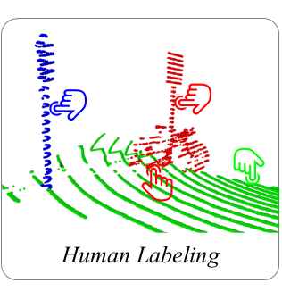
Pre-segmentation yields three components colored in red, blue, and green.
Coarsely labeling all components ensures minimal chance of missing underrepresented instances as they cover the majority of points.
3.6 Types of labels
Based on the components proposals, we can obtain three type of labels:
- Sparse labels: These labels are obtained directly from the points that have been annotated by human annotators. Although only a small subset of points are labeled, sparse labels provide the most accurate and diverse form of supervision.
- Weak labels: Weak labels are derived from the human-annotated sparse labels within each component. For example, in the previous figure showcasing human labels, all red points can only belong to either the bicycle or traffic sign category. We distribute weak labels from each component to the points contained within it. These multi-category weak labels offer less precise supervision but are more densely distributed, covering a larger portion of points.
- Propagated labels: Propagated labels are applicable to components that contain only one category. Similar to the pre-segmentation approach, the propagated labels span a wide range of points. However, since certain categories may be easier to separate and more likely to form distinct components, the distribution of the propagated labels may be biased and less diverse compared to the sparse labels.
By employing these different types of labels, we are able to leverage various levels of supervision and cover a significant portion of points within the LiDAR data. Each type of label offers its own strengths and limitations, contributing to a more comprehensive understanding of the data for the segmentation task.
Then, we formulate a joint loss function by exploiting the three types of labels:
\(L = L_{sparse} + L_{propagated} + L_{weak}\)
where \(L_{sparse}\) and \(L_{propagated}\) are weighted cross-entropy loss with respect to the sparse labels and propagated labels, respectively. We utilize the inverse square root of the label frequency as category weights to emphasize the underrepresented categories.
In other hand, we denote weak labels as binary mask \(l_{ij}\) for point \(i\) and category \(j\). \(l_{ij} = 1\) when point \(i\) belongs to component that contains category \(j\). We exploit the multi-category weak labels by penalizing the impossible predictions. \(P_{ij}\) is the predicted probability of point \(i\), and \(n\) is the number of points.
\(L_{weak} = -\tfrac{1}{n}\sum_{i=1}^{n}log(1\:\:-\:\:\sum_{l_{ij=0}}^{}p_{ij})\)
This loss term ensures that the model learns to avoid assigning probabilities to categories that should not be present in the corresponding components. By incorporating these loss terms, we encourage the model to effectively utilize the different types of labels and improve the overall segmentation performance.
3.7 Contrastive protype learning
Contrastive learning is a powerful technique for both supervised learning and few-shot learning. It offers several advantages over the traditional cross-entropy loss, such as addressing issues like poor margins and enabling the construction of a more detailed embedding space.
To leverage contrastive learning, I adopt a strategy where I learn the class prototypes, denoted as Pc, through a moving average process over multiple iterations. The computation is defined as follows:
\(P_{c} \gets mP_{c}\:+\:(1 -m)\tfrac{1}{n_{c}}\sum_{y_{i=c}}^{}stopgrad(h(f(x_{i})))\)
where \(f\left( x_{i} \right)\) is the embedding of point \(x_{i}\), \(h\) is a linear projection head with vector normalization, stopgrad denotes the stop gradient operation, \({y_{i}}\) is the label of \(x_{i}\), \(n_{c}\) is the number of points with label \(c\) in a batch, and \(m\) is a momentum coefficient. In the beginning, \(P_{c}\) are initialized randomly.
To calculate the prototype loss, denoted as Lproto, I consider the points with both sparse labels and propagated labels within each batch. The computation is defined as:
\(L_{proto} = \tfrac{1}{n}\sum_{i}^{n}-w_{yi}\:\:log \tfrac{exp(h(f_{xi})).P_{yi}/\tau)}{\sum_{c}^{}exp(h(f(x_{i})).P_{c}/\tau)}\)
where \(h(f_{xi})).P_{yi}\) indicates the cosine similarity between the projected embedding and the prototype, \(τ\) is a temperature hyper-parameter, \(n\) is the number of points, and \(w_{yi}\) is the inverse square root weight of category \(y_{i}\).
Through this prototype loss, we encourage the model to better align the projected embeddings with the corresponding prototypes, leveraging the cosine similarity.
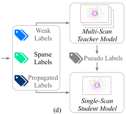
3.8 Multi-scan distillation
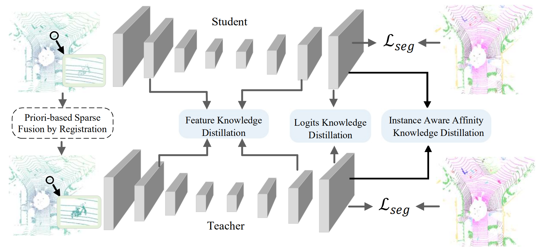
Our goal is to develop a segmentation network that can efficiently process single LiDAR scans and be deployed in real-time onboard applications. In our label-efficient training approach, we train a multi-scan network as a teacher model. This teacher model incorporates temporal fusion of multiple scans and takes the densified point cloud as input, compensating for the sparsity and incompleteness typically observed within a single scan.
The teacher model is expected to harness the richer semantics provided by multiple scans and exhibit improved performance compared to a single-scan model. This is particularly beneficial for addressing underrepresented categories, which often have smaller and sparser instances. Subsequently, we transfer the knowledge from the multi-scan teacher model to enhance the performance of the single-scan student model.
The student model shares the same backbone network as the teacher model and is initially trained from scratch using the same approach, with the exception that it processes single-scan inputs. We then align the student model’s predictions with the soft pseudo-labels generated by the teacher model using cross-entropy loss.
The eauation for the distillation loss is:
\(L_{dis} = -\tfrac{T^{2}}{n}\sum_{i}^{n}\sum_{c}^{}\tfrac{exp(u_{ic}/T)}{\sum_{c'}^{}exp(u_{ic'}/T)}log(\tfrac{exp(v_{ic}/T)}{\sum_{c'}^{}exp(v_{ic'}/T)})\)
where \(u_{ic}\) and \(v_{ic}\) are the predicted logits for point \(i\) and category \(c\) by the teacher and student models respectively, and \(T\) is a temperature hyper-parameter. A higher temperature is typically used so that the probability distribution across classes is smoother, and the distillation is thus encouraged to match the negative logits, which also contain rich information. The cross-entropy is multiplied by \(T^{2}\) to ensure the gradients’ magnitudes are aligned with other existing losses.
It is important to note that the idea of multi-scan distillation is specifically advantageous for our label-efficient LiDAR segmentation setting. In fully supervised settings, where all labels are already available and accurate, there is no need to rely on pseudo labels. Similarly, for indoor settings where points are sampled from high-quality reconstructed meshes, the use of a multi-scan teacher model is unnecessary.
4. Experiments
4.1 Setup
Authors choose Cylinder3D as our backbone network, which is a recent and highly advanced method for LiDAR semantic segmentation. To mimic the obtained human annotations, we utilize ground truth labels without introducing any additional noise.
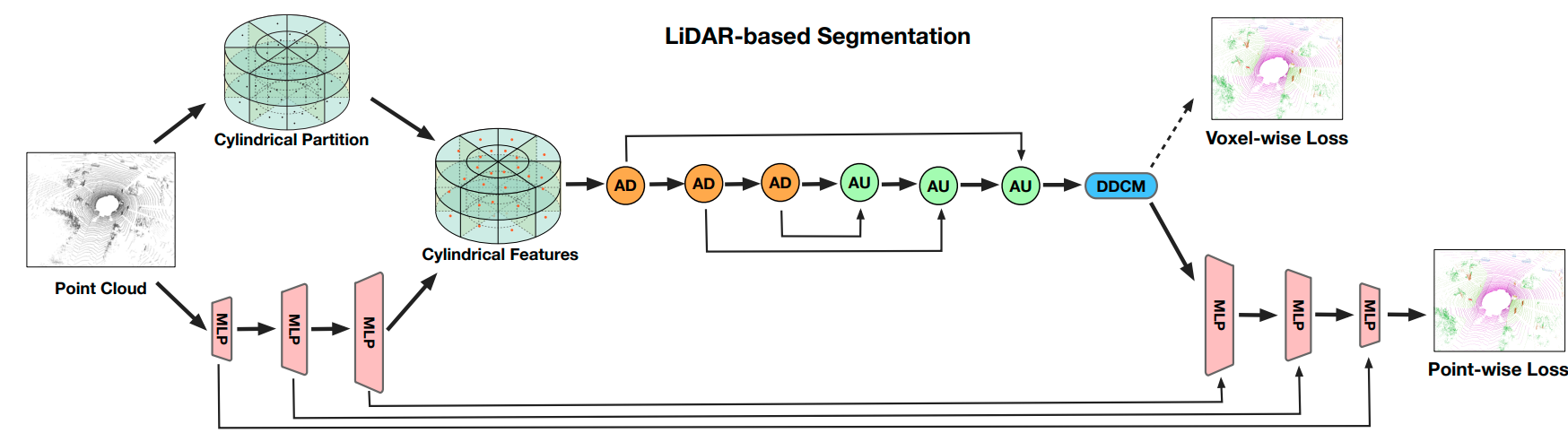
Overall framework of the Cylinder3D for LiDAR segmentation.
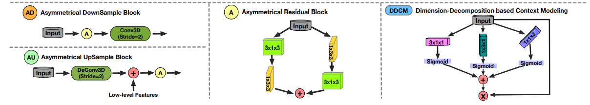
The top half of the figure presents an overview of the Cylinder3D pipeline. It starts with the input of the LiDAR point cloud into a Multi-Layer Perceptron (MLP) to extract features on a point-wise basis. These features are then reassigned based on cylindrical partitioning. Asymmetrical 3D convolution networks are employed to generate voxel-wise outputs. Finally, a point-wise module is introduced to refine these outputs further.
The bottom half of the figure elaborates on four key components: the Asymmetrical Downsample block (AD), Asymmetrical Upsample block (AU), Asymmetrical residual block (A), and Dimension-Decomposition based Context Modeling (DDCM). These components contribute to the effectiveness and performance of the Cylinder3D network architecture.
4.2 Comparison on SemanticKITTI
In our evaluation, we compare the proposed method with both fully supervised approaches (top half) and label-efficient methods (bottom half).
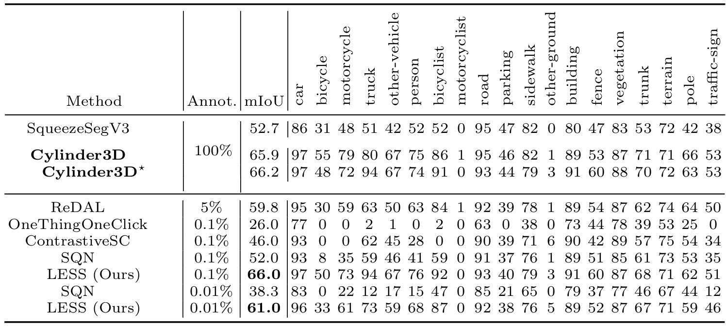
Comparison on SemanticKITTI validation set.
It is important to note that all competing label-efficient methods primarily focus on indoor settings and are not specifically tailored for outdoor LiDAR segmentation.
The results demonstrate that even with only 0.1% sparse labels, our proposed method achieves comparable performance to the fully supervised baseline, Cylinder3D. This remarkable performance showcases the potential of our approach for real-world applications. Upon analyzing the breakdown results, we observe that the variations between the methods mainly stem from the underrepresented categories, such as bicycles, motorcycles, persons, and bicyclists. These categories pose challenges due to their smaller instances and lower occurrence frequency.
4.3 Comparison on nuScene & ablation study
In our study, authors wanted to provide a fair comparison by training the Cylinder3D model from scratch, as the author-released model was pre-trained on the SemanticKITTI dataset.
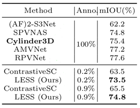
For other fully-supervised methods (top half), we obtained the results either from the literature or through correspondence with the authors.
Since no previous label-efficient methods were tested on the nuScenes dataset, we adapted the source code published by the authors to train ContrastiveSceneContext [23] from scratch. Our proposed method demonstrates superior performance compared to ContrastiveSceneContext by a significant margin. Even with only 0.2% sparse labels, the results are highly competitive with the fully-supervised counterpart.
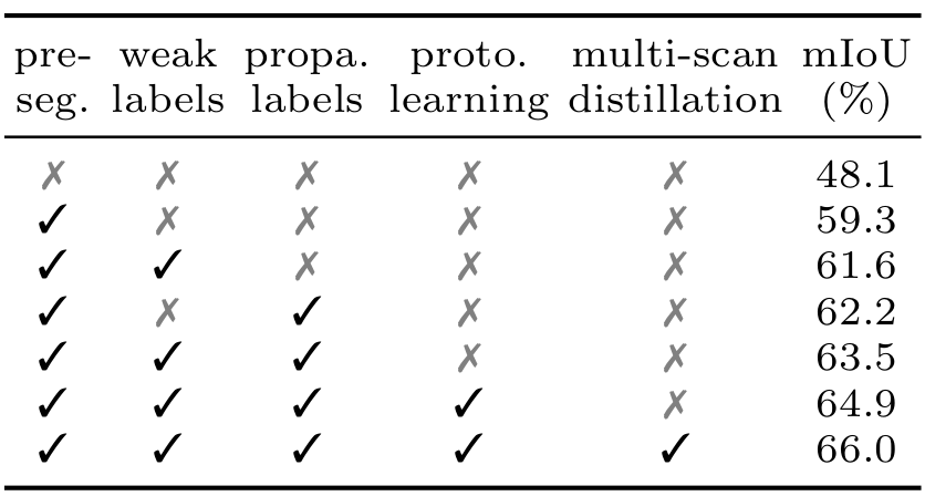
The right figure in our study presents the results of an ablation study, where we evaluate the impact of each individual component. When incorporating all the aforementioned components, we achieve a mIoU result of 66.0%. It is worth noting that both contrastive prototype learning and multi-scan distillation further enhance the performance and effectively narrow the gap between our proposed method (LESS) and the fully-supervised counterpart in terms of mIoU. These two proposed components play a crucial role in improving the accuracy of underrepresented categories.
4.4 Analysis of multi-scan distillation
The teacher model leverages the densified point clouds through temporal fusion, leading to improved performance compared to the single-scan model, including the fully supervised single-scan model. By distilling knowledge from the teacher model, the student model exhibits significant improvements, particularly in underrepresented classes, and achieves the same mIoU as the fully supervised model.
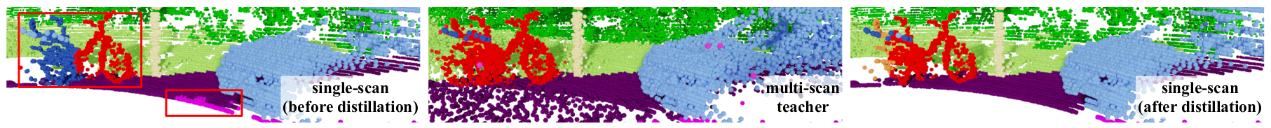
The multi-scan teacher leverages the richer semantics via temporal fusion to accurately segment the bicycle and ground, which provides high-quality supervision to enhance the single-scan model.
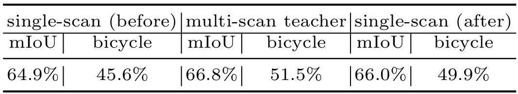
Results of the multi-scan distillation on the SemanticKITTI validation set. 0.1% annotations are used.
Upon examining the figure provided above, we can observe a slight improvement in the mIoU result for the underrepresented category of bicycles when utilizing the multi-scan teacher model.
4.5 Qualitative results
When analyzing the output, it said that red rectangles indicating incorrect predictions. Our results are comparable to those of the fully supervised approach, demonstrating the effectiveness of our method. However, it is worth noting that ContrastiveSceneContext, a different approach, yields inferior results, particularly in underrepresented categories such as persons and bicycles. These categories exhibit more prominent errors in the predictions made by ContrastiveSceneContext.
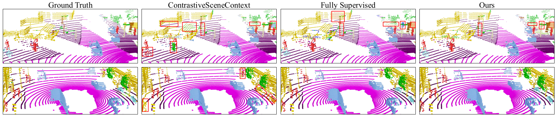
Qualitative examples on the SemanticKITTI (first row) and nuScenes (second row) validation sets.
5. Conclusion and feature works
In conclusion, I would like to provide the following comments and suggestions for future work:
- This paper is first hands-on paper which focused label-efficient semantic segmentation in outdoor setting.This paper represents our firsthand exploration of label-efficient semantic segmentation in outdoor settings, filling a gap in the existing research literature.
- Proposed approach achieves accuracy levels comparable to fully supervised methods, even with coarse labeling, in common categories such as cars, roads, and vegetation.
- Notably, I observed significant improvements in the underrepresented categories by incorporating knowledge distillation. Moving forward, it would be interesting to investigate novel techniques to address the sparsity present in LiDAR data, such as point cloud upsampling or densification methods, to enhance the accuracy and completeness of semantic segmentation. Additionally, I am intrigued by the potential results of applying the proposed LESS method in conjunction with the state-of-the-art FusionDepth method, which was recently presented by one of our colleagues during our seminar.
- Regarding future works, it would be beneficial to explore the potential of leveraging state-of-the-art FusionDepth methods in conjunction with the proposed LESS method. By combining these approaches, we can potentially enhance the accuracy and robustness of semantic segmentation, especially in challenging scenarios.
- It is worth noting that the underrepresented categories, such as humans and motorcycles, are less prevalent in countries with less chaotic traffic situations, like Germany and Singapore, where the SemanticKITTI and nuScenes datasets were collected. To gain a more comprehensive understanding, future data collection efforts could be conducted in environments with more chaotic traffic conditions, such as in India, where there are dense streets and a large number of motorized two-wheelers.
- Proposed label-efficient methods, particularly when applied to synthetic data [16], offer an opportunity to explore and address the challenges posed by underrepresented traffic agents. This is in contrast to the limitations of existing real-world datasets, such as nuScenes or KITTI, which may not fully capture the complexities and intricacies of real-world environments. By leveraging synthetic data, we can augment the dataset with diverse traffic scenarios and simulate a more comprehensive representation of the real world, enabling more robust and accurate evaluation of label-efficient methods.
- It is important to highlight that there are no similar works available for direct comparison with the results of other researchers. This further emphasizes the novelty and uniqueness of our approach within the field of label-efficient semantic segmentation.
6. References
[1] Behley, J., Garbade, M.: Semantickitti: A dataset for semantic scene understanding of lidar sequences. ICCV(2019)
[2] Caesar, H., Bankiti, V.: nuscenes: A multimodal dataset for autonomous driving. CVPR(2020)
[3] Zhu, X., Zhou, H. : Cylindrical and asymmetrical 3d convolution networks for lidar segmentation. CVPR(2021)
[4] Xu, J., Zhang, R. : Rpvnet: A deep and ecient range-point-voxel fusion network for lidar point cloud segmentation, arXiv preprint(2021)
[5] Cheng, R., Razani, R.: Af2-s3net: Attentive feature fusion with adaptive feature selection for sparse semantic segmentation network. CVPR(2021)
[6] Dai, A., Niessner, M.: Scannet: Richly-annotated 3d reconstructions of indoor scenes. CVPR (2017)
[7] Chang, A., X., Funkhouser: Shapenet: An information-rich 3d model repository. arXiv preprint (2015)
[8] Vizzo, I., Stachniss, C.: Rangenet++: Fast and accurate lidar semantic segmentation. IEEE(2019)
[9] Hu, Q., Yang, B. : Randla-net: Efficient semantic segmentation of large-scale point clouds. CVPR (2020)
[10] Shi, X., Xu, X.: Label-efficient point cloud semantic segmentation: An active learning approach. arXiv:2101.06931 (2021)
[11] Hou, J., Niessner, M. : Exploring data-efficient 3d scene understanding with contrastive scene contexts. CVPR(2021)
[12] Liu, Z., Qi: One thing one click: A self-training approach for weakly supervised 3d semantic segmentation. CVPR(2021)
[13] Xu, X., Lee, G.H.: Weakly supervised semantic point cloud segmentation: Towards10x fewer labels. CVPR(2020)
[14] Gao, Y., Fei, N. : Contrastive prototype learning with augmented embeddings for few-shot learning. arXiv:2101.09499 (2021)
[15] Qiu, S., Jiang, F.: Multi-to-Single Knowledge Distillation for Point Cloud Semantic Segmentation. CVPR(2023)
[16] Sun, T., Tombari, F.: SHIFT: A Synthetic Driving Dataset for Continuous Multi-Task Domain Adaptation. CVPR(2022)
7. Annex
7.1 Dataset
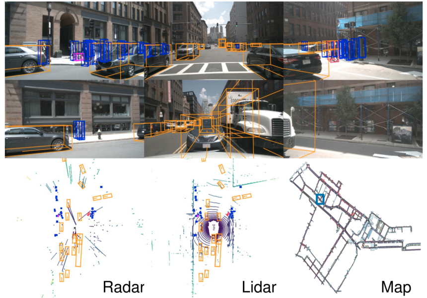
- The nuScenes dataset, collected in Boston and Singapore, exhibits sparser point clouds compared to the SemanticKITTI dataset from Germany.
- In nuScenes, only 2 scans per second are labeled, whereas in SemanticKITTI, 10 scans per second receive labels.
- The discrepancy in sensor technology, specifically the use of 32-beam and 64-beam sensors, contributes to the significant difference in the number of points per scan between nuScenes (26k points) and SemanticKITTI (120k points). As a possible answer for the one of the question during the Q&A time: Notable differences between the nuScenes dataset, collected in Boston and Singapore, and the SemanticKITTI dataset from Germany. The point clouds in nuScenes are sparser compared to SemanticKITTI. Moreover, while SemanticKITTI labels 10 scans per second, nuScenes only labels 2 scans per second. These variations in labeling frequency reflect the different approaches taken in the data collection process. Additionally, the dissimilarity in sensor technology, specifically the use of 32-beam and 64-beam sensors, contributes to the substantial difference in the number of points per scan. These factors underline the distinctions and challenges associated with these datasets and should be considered when evaluating and comparing segmentation methods.
7.2 Network training
- Trained on 4 Nvidia A100 GPUs
- Batch size:12 for the single-scan, and 8 for the multi-scan
- Optimizer: Adam
- Learning rate: 1e-3, then decated 1e-4 after convergence.
- During distillation, learning rate: 1e-4
- Other training parameters are the same as Cylinder3D [3]
7.3 Visual results of pre-segmentation
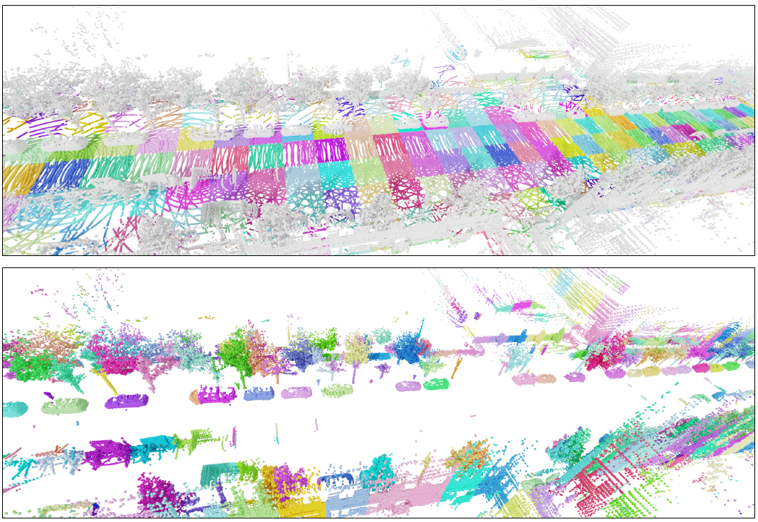
In the first row of the provided visualization, we can observe the detected ground points within each cell. The non-ground points are highlighted in gray, distinguishing them from the ground points.
Insecond row, we see the connected components of these non-ground points. Each distinct color represents a different connected component. It is important to note that this particular example is taken from the nuScenes dataset, where 40 scans have been fused together to generate these visualizations.